
PySpark Dataframe Basics
In this post, I will use a toy data to show some basic dataframe operations that are helpful in working with dataframes in PySpark or tuning the performance of Spark jobs. The list is by no means exhaustive, but they are the most common ones I used.
I’m using Spark 2.1.1, so there may be new functionalities not in this post as the latest version is 2.3.0. You can find all of the current dataframe operations in the source code and the API documentation.
Dataframe basics for PySpark
Spark has moved to a dataframe API since version 2.0. A dataframe in Spark is similar to a SQL table, an R dataframe, or a pandas dataframe. In Spark, dataframe is actually a wrapper around RDDs, the basic data structure in Spark. In my opinion, however, working with dataframes is easier than RDD most of the time.
There are a few ways to read data into Spark as a dataframe. In this post, I will load the first few rows of Titanic data on Kaggle into a pandas dataframe, then convert it into a Spark dataframe.
import findspark
findspark.init()
import pyspark # only run after findspark.init()
from pyspark.sql import SparkSession
spark = SparkSession.builder.getOrCreate()
import pandas as pd
sc = spark.sparkContext
Make a sample dataframe from Titanic data
data1 = {'PassengerId': {0: 1, 1: 2, 2: 3, 3: 4, 4: 5},
         'Name': {0: 'Owen', 1: 'Florence', 2: 'Laina', 3: 'Lily', 4: 'William'},
         'Sex': {0: 'male', 1: 'female', 2: 'female', 3: 'female', 4: 'male'},
         'Survived': {0: 0, 1: 1, 2: 1, 3: 1, 4: 0}}

data2 = {'PassengerId': {0: 1, 1: 2, 2: 3, 3: 4, 4: 5},
         'Age': {0: 22, 1: 38, 2: 26, 3: 35, 4: 35},
         'Fare': {0: 7.3, 1: 71.3, 2: 7.9, 3: 53.1, 4: 8.0},
         'Pclass': {0: 3, 1: 1, 2: 3, 3: 1, 4: 3}}

df1_pd = pd.DataFrame(data1, columns=data1.keys())
df2_pd = pd.DataFrame(data2, columns=data2.keys())
df1_pd
| PassengerId | Name | Sex | Survived | |
|---|---|---|---|---|
| 0 | 1 | Owen | male | 0 |
| 1 | 2 | Florence | female | 1 |
| 2 | 3 | Laina | female | 1 |
| 3 | 4 | Lily | female | 1 |
| 4 | 5 | William | male | 0 |
df2_pd
| PassengerId | Age | Fare | Pclass | |
|---|---|---|---|---|
| 0 | 1 | 22 | 7.3 | 3 |
| 1 | 2 | 38 | 71.3 | 1 |
| 2 | 3 | 26 | 7.9 | 3 |
| 3 | 4 | 35 | 53.1 | 1 |
| 4 | 5 | 35 | 8.0 | 3 |
Convert pandas dataframe to Spark dataframe
df1 = spark.createDataFrame(df1_pd)
df2 = spark.createDataFrame(df2_pd)
df1.show()
+-----------+--------+------+--------+
|PassengerId|    Name|   Sex|Survived|
+-----------+--------+------+--------+
|          1|    Owen|  male|       0|
|          2|Florence|female|       1|
|          3|   Laina|female|       1|
|          4|    Lily|female|       1|
|          5| William|  male|       0|
+-----------+--------+------+--------+
df1.printSchema()
root
 |-- PassengerId: long (nullable = true)
 |-- Name: string (nullable = true)
 |-- Sex: string (nullable = true)
 |-- Survived: long (nullable = true)
Basic dataframe verbs
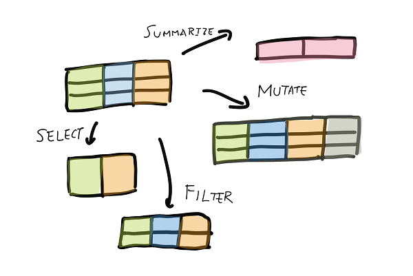
In R’s dplyr package, Hadley Wickham defined the 5 basic verbs — select, filter, mutate, summarize, and arrange. Here are the equivalents of the 5 basic verbs for Spark dataframes.
Select
I can select a subset of columns. The method select() takes either a list of column names or an unpacked list of names.
cols1 = ['PassengerId', 'Name']
df1.select(cols1).show()
+-----------+--------+
|PassengerId|    Name|
+-----------+--------+
|          1|    Owen|
|          2|Florence|
|          3|   Laina|
|          4|    Lily|
|          5| William|
+-----------+--------+
Filter
I can filter a subset of rows. The method filter() takes column expressions or SQL expressions. Think of the WHERE clause in SQL queries.
- Filter with a column expression
df1.filter(df1.Sex == 'female').show()
+-----------+--------+------+--------+
|PassengerId|    Name|   Sex|Survived|
+-----------+--------+------+--------+
|          2|Florence|female|       1|
|          3|   Laina|female|       1|
|          4|    Lily|female|       1|
+-----------+--------+------+--------+
- Filter with a SQL expression. Note the double and single quotes as I’m passing a SQL where clause into
filter().
df1.filter("Sex='female'").show()
+-----------+--------+------+--------+
|PassengerId|    Name|   Sex|Survived|
+-----------+--------+------+--------+
|          2|Florence|female|       1|
|          3|   Laina|female|       1|
|          4|    Lily|female|       1|
+-----------+--------+------+--------+
Mutate, or creating new columns
I can create new columns in Spark using .withColumn(). I have yet found a convenient way to create multiple columns at once without chaining multiple .withColumn() methods.
df2.withColumn('AgeTimesFare', df2.Age*df2.Fare).show()
+-----------+---+----+------+------------+
|PassengerId|Age|Fare|Pclass|AgeTimesFare|
+-----------+---+----+------+------------+
|          1| 22| 7.3|     3|       160.6|
|          2| 38|71.3|     1|      2709.4|
|          3| 26| 7.9|     3|       205.4|
|          4| 35|53.1|     1|      1858.5|
|          5| 35| 8.0|     3|       280.0|
+-----------+---+----+------+------------+
Summarize and group by
To summarize or aggregate a dataframe, first I need to convert the dataframe to a GroupedData object with groupby(), then call the aggregate functions.
gdf2 = df2.groupby('Pclass')
gdf2
<pyspark.sql.group.GroupedData at 0x9bc8f28>
I can take the average of columns by passing an unpacked list of column names.
avg_cols = ['Age', 'Fare']
gdf2.avg(*avg_cols).show()
+------+------------------+-----------------+
|Pclass|          avg(Age)|        avg(Fare)|
+------+------------------+-----------------+
|     1|              36.5|             62.2|
|     3|27.666666666666668|7.733333333333333|
+------+------------------+-----------------+
To call multiple aggregation functions at once, pass a dictionary.
gdf2.agg({'*': 'count', 'Age': 'avg', 'Fare':'sum'}).show()
+------+--------+------------------+---------+
|Pclass|count(1)|          avg(Age)|sum(Fare)|
+------+--------+------------------+---------+
|     1|       2|              36.5|    124.4|
|     3|       3|27.666666666666668|     23.2|
+------+--------+------------------+---------+
To rename the columns count(1), avg(Age) etc, use toDF().
(
    gdf2
    .agg({'*': 'count', 'Age': 'avg', 'Fare':'sum'})
    .toDF('Pclass', 'counts', 'average_age', 'total_fare')
    .show()
)
+------+------+------------------+----------+
|Pclass|counts|       average_age|total_fare|
+------+------+------------------+----------+
|     1|     2|              36.5|     124.4|
|     3|     3|27.666666666666668|      23.2|
+------+------+------------------+----------+
Arrange (sort)
Use the .sort() method to sort the dataframes. I haven’t seen a good use case for this in Spark though.
df2.sort('Fare', ascending=False).show()
+-----------+---+----+------+
|PassengerId|Age|Fare|Pclass|
+-----------+---+----+------+
|          2| 38|71.3|     1|
|          4| 35|53.1|     1|
|          5| 35| 8.0|     3|
|          3| 26| 7.9|     3|
|          1| 22| 7.3|     3|
+-----------+---+----+------+
Joins and unions
There are two ways to combine dataframes — joins and unions. The idea here is the same as joining and unioning tables in SQL.
Joins
For example, I can join the two titanic dataframes by the column PassengerId
df1.join(df2, ['PassengerId']).show()
+-----------+--------+------+--------+---+----+------+
|PassengerId|    Name|   Sex|Survived|Age|Fare|Pclass|
+-----------+--------+------+--------+---+----+------+
|          5| William|  male|       0| 35| 8.0|     3|
|          1|    Owen|  male|       0| 22| 7.3|     3|
|          3|   Laina|female|       1| 26| 7.9|     3|
|          2|Florence|female|       1| 38|71.3|     1|
|          4|    Lily|female|       1| 35|53.1|     1|
+-----------+--------+------+--------+---+----+------+
I can also join by conditions, but it creates duplicate column names if the keys have the same name, which is frustrating. For now, the only way I know to avoid this is to pass a list of join keys as in the previous cell. If I want to make nonequi joins, then I need to rename the keys before I join.
Nonequi joins
Here is an example of nonequi join. They can be very slow due to skewed data, but this is one thing that Spark can do that Hive can not.
df1.join(df2, df1.PassengerId <= df2.PassengerId).show() # Note the duplicate col names
+-----------+--------+------+--------+-----------+---+----+------+
|PassengerId|    Name|   Sex|Survived|PassengerId|Age|Fare|Pclass|
+-----------+--------+------+--------+-----------+---+----+------+
|          1|    Owen|  male|       0|          1| 22| 7.3|     3|
|          1|    Owen|  male|       0|          2| 38|71.3|     1|
|          1|    Owen|  male|       0|          3| 26| 7.9|     3|
|          1|    Owen|  male|       0|          4| 35|53.1|     1|
|          1|    Owen|  male|       0|          5| 35| 8.0|     3|
|          2|Florence|female|       1|          2| 38|71.3|     1|
|          2|Florence|female|       1|          3| 26| 7.9|     3|
|          2|Florence|female|       1|          4| 35|53.1|     1|
|          2|Florence|female|       1|          5| 35| 8.0|     3|
|          3|   Laina|female|       1|          3| 26| 7.9|     3|
|          3|   Laina|female|       1|          4| 35|53.1|     1|
|          3|   Laina|female|       1|          5| 35| 8.0|     3|
|          4|    Lily|female|       1|          4| 35|53.1|     1|
|          4|    Lily|female|       1|          5| 35| 8.0|     3|
|          5| William|  male|       0|          5| 35| 8.0|     3|
+-----------+--------+------+--------+-----------+---+----+------+
Unions
Union() returns a dataframe from the union of two dataframes
df1.union(df1).show()
+-----------+--------+------+--------+
|PassengerId|    Name|   Sex|Survived|
+-----------+--------+------+--------+
|          1|    Owen|  male|       0|
|          2|Florence|female|       1|
|          3|   Laina|female|       1|
|          4|    Lily|female|       1|
|          5| William|  male|       0|
|          1|    Owen|  male|       0|
|          2|Florence|female|       1|
|          3|   Laina|female|       1|
|          4|    Lily|female|       1|
|          5| William|  male|       0|
+-----------+--------+------+--------+
Some of my iterative algorithms create chained union() objects. There is a potential catch that the execution plan may grow too long, which cause performance problems or errors.
One common symptom of performance issues caused by chained unions in a for loop is it took longer and longer to iterate through the loop. In this case, repartition() and checkpoint() may help solving this problem.
Dataframe input and output (I/O)
There are two classes pyspark.sql.DataFrameReader and pyspark.sql.DataFrameWriter that handles dataframe I/O. Depending on the configuration, the files may be saved locally, through a Hive metasore, or to a Hadoop file system (HDFS).
Common methods on saving dataframes to files include saveAsTable() for Hive tables and saveAsFile() for local or Hadoop file system.
I will refer to the documentation for examples on how to read and write dataframes for different formats.
The spark.sql API
Many of the operations that I showed can be accessed by writing SQL (Hive) queries in spark.sql(). This is also a convenient way to read Hive tables into Spark dataframes. To make an existing Spark dataframe usable for spark.sql(), I need to register said dataframe as a temporary table.
Temp tables
As an example, I can register the two dataframes as temp tables then join them through spark.sql().
df1.createOrReplaceTempView('df1_temp')
df2.createOrReplaceTempView('df2_temp')
query = '''
    select
        a.PassengerId,
        a.Name,
        a.Sex,
        a.Survived,
        b.Age,
        b.Fare,
        b.Pclass
    from df1_temp a
    join df2_temp b
        on a.PassengerId = b.PassengerId'''
dfj = spark.sql(query)
dfj.show()
+-----------+--------+------+--------+---+----+------+
|PassengerId|    Name|   Sex|Survived|Age|Fare|Pclass|
+-----------+--------+------+--------+---+----+------+
|          5| William|  male|       0| 35| 8.0|     3|
|          1|    Owen|  male|       0| 22| 7.3|     3|
|          3|   Laina|female|       1| 26| 7.9|     3|
|          2|Florence|female|       1| 38|71.3|     1|
|          4|    Lily|female|       1| 35|53.1|     1|
+-----------+--------+------+--------+---+----+------+
Going deeper

In this section, I will go through some idea and useful tools associated with said ideas that I found helpful in tuning performance or debugging dataframes. The first of which is the difference between two types of operations: transformations and actions, and a method explain() that prints out the execution plan of a dataframe.
Explain(), transformations, and actions
When I create a dataframe in PySpark, dataframes are lazy evaluated. What it means is that most operations are transformations that modify the execution plan on how Spark should handle the data, but the plan is not executed unless we call an action.
For example, if I want to join df1 and df2 on the key PassengerId as before:
df1.explain()
== Physical Plan ==
Scan ExistingRDD[PassengerId#0L,Name#1,Sex#2,Survived#3L]
df2.explain()
== Physical Plan ==
Scan ExistingRDD[PassengerId#9L,Age#10L,Fare#11,Pclass#12L]
dfj1 = df1.join(df2, ['PassengerId'])
dfj1.explain()
== Physical Plan ==
*Project [PassengerId#0L, Name#1, Sex#2, Survived#3L, Age#10L, Fare#11, Pclass#12L]
+- *SortMergeJoin [PassengerId#0L], [PassengerId#9L], Inner
   :- *Sort [PassengerId#0L ASC NULLS FIRST], false, 0
   :  +- Exchange hashpartitioning(PassengerId#0L, 200)
   :     +- *Filter isnotnull(PassengerId#0L)
   :        +- Scan ExistingRDD[PassengerId#0L,Name#1,Sex#2,Survived#3L]
   +- *Sort [PassengerId#9L ASC NULLS FIRST], false, 0
      +- Exchange hashpartitioning(PassengerId#9L, 200)
         +- *Filter isnotnull(PassengerId#9L)
            +- Scan ExistingRDD[PassengerId#9L,Age#10L,Fare#11,Pclass#12L]
In this case, join() is a transformation that laid out a plan for Spark to join the two dataframes, but it wasn’t executed unless I call an action, such as .count(), that has to go through the actual data defined by df1 and df2 in order to return a Python object (integer).
dfj1.count()
5
What if I join the two dataframes through the spark.sql() API instead of calling .join()? In this case, both happen to generate the same execution plan. But it’s not always like this. A good execution plan equals good performance, and I explain() a lot when I need to tune performance of Spark jobs.
query = '''
    select
        a.PassengerId,
        a.Name,
        a.Sex,
        a.Survived,
        b.Age,
        b.Fare,
        b.Pclass
    from df1_temp a
    join df2_temp b
        on a.PassengerId = b.PassengerId'''
dfj = spark.sql(query)
dfj.explain()
== Physical Plan ==
*Project [PassengerId#0L, Name#1, Sex#2, Survived#3L, Age#10L, Fare#11, Pclass#12L]
+- *SortMergeJoin [PassengerId#0L], [PassengerId#9L], Inner
   :- *Sort [PassengerId#0L ASC NULLS FIRST], false, 0
   :  +- Exchange hashpartitioning(PassengerId#0L, 200)
   :     +- *Filter isnotnull(PassengerId#0L)
   :        +- Scan ExistingRDD[PassengerId#0L,Name#1,Sex#2,Survived#3L]
   +- *Sort [PassengerId#9L ASC NULLS FIRST], false, 0
      +- Exchange hashpartitioning(PassengerId#9L, 200)
         +- *Filter isnotnull(PassengerId#9L)
            +- Scan ExistingRDD[PassengerId#9L,Age#10L,Fare#11,Pclass#12L]
Data persistence: cache() and checkpoint()
caching
Proper caching is the key to high performance Spark. But to be honest, I still don’t have good intuition on when to cache and when not to cache. I do know a rule of thumb that
- Cache a dataframe when it is used multiple times in the script.
Keep in mind that a dataframe only cached after the first action such as saveAsTable(). If for whatever reason I want to make sure the data is cached before I save the dataframe, then I have to call an action like .count() before I save it.
df1.cache()
DataFrame[PassengerId: bigint, Name: string, Sex: string, Survived: bigint]
This also works as .cache() is an inplace method.
df1 = df1.cache()
To check if a dataframe is cached, check the storageLevel property.
df1.storageLevel
StorageLevel(True, True, False, True, 1)
To un-cache a dataframe, use unpersist()
df1.unpersist()
df1.storageLevel
StorageLevel(False, False, False, False, 1)
There are 4 caching levels that can be fine-tuned with persist(), but I have not seen a use case where fine tuning has been worthwhile. Refer to the persist() documentation for detail.
Checkpointing
I said that sometimes chaining too many union() cause performance problem or even out of memory errors. checkpoint() truncates the execution plan and saves the checkpointed dataframe to a temporary location on the disk.
Jacek Laskowski recommends caching before checkpointing so Spark doesn’t have to read in the dataframe from disk after it’s checkpointed.
To use checkpoint(), I need to specify the temporary file location to save the datafame to by accessing the sparkContext object from SparkSession.
sc = spark.sparkContext
sc.setCheckpointDir("/checkpointdir") # save to c:/checkpointdir
For example, I can join df1 to itself 3 times:
df = df1.join(df1, ['PassengerId'])
df.join(df1, ['PassengerId']).explain()
== Physical Plan ==
*Project [PassengerId#0L, Name#1, Sex#2, Survived#3L, Name#287, Sex#288, Survived#289L, Name#299, Sex#300, Survived#301L]
+- *SortMergeJoin [PassengerId#0L], [PassengerId#298L], Inner
   :- *Project [PassengerId#0L, Name#1, Sex#2, Survived#3L, Name#287, Sex#288, Survived#289L]
   :  +- *SortMergeJoin [PassengerId#0L], [PassengerId#286L], Inner
   :     :- *Sort [PassengerId#0L ASC NULLS FIRST], false, 0
   :     :  +- Exchange hashpartitioning(PassengerId#0L, 200)
   :     :     +- *Filter isnotnull(PassengerId#0L)
   :     :        +- Scan ExistingRDD[PassengerId#0L,Name#1,Sex#2,Survived#3L]
   :     +- *Sort [PassengerId#286L ASC NULLS FIRST], false, 0
   :        +- Exchange hashpartitioning(PassengerId#286L, 200)
   :           +- *Filter isnotnull(PassengerId#286L)
   :              +- Scan ExistingRDD[PassengerId#286L,Name#287,Sex#288,Survived#289L]
   +- *Sort [PassengerId#298L ASC NULLS FIRST], false, 0
      +- Exchange hashpartitioning(PassengerId#298L, 200)
         +- *Filter isnotnull(PassengerId#298L)
            +- Scan ExistingRDD[PassengerId#298L,Name#299,Sex#300,Survived#301L]
I can also checkpoint() after the first join to truncate the plan.
df = df1.join(df1, ['PassengerId']).checkpoint()
df.join(df1, ['PassengerId']).explain()
== Physical Plan ==
*Project [PassengerId#0L, Name#1, Sex#2, Survived#3L, Name#314, Sex#315, Survived#316L, Name#335, Sex#336, Survived#337L]
+- *SortMergeJoin [PassengerId#0L], [PassengerId#334L], Inner
   :- *Filter isnotnull(PassengerId#0L)
   :  +- Scan ExistingRDD[PassengerId#0L,Name#1,Sex#2,Survived#3L,Name#314,Sex#315,Survived#316L]
   +- *Sort [PassengerId#334L ASC NULLS FIRST], false, 0
      +- Exchange hashpartitioning(PassengerId#334L, 200)
         +- *Filter isnotnull(PassengerId#334L)
            +- Scan ExistingRDD[PassengerId#334L,Name#335,Sex#336,Survived#337L]
Partitions and repartition()
Another common cause of performance problems for me was having too many partitions. I think the Hadoop world call this the small file problem. A rule of thumb, which I first heard from these slides, is
- Keep the partitions to ~128MB.
In PySpark, however, there is no way to infer the size of the dataframe partitions. In my experience, as long as the partitions are not 10KB or 10GB but are in the order of MBs, then the partition size shouldn’t be too much of a problem.
To check the number of partitions, use .rdd.getNumPartitions()
df1.rdd.getNumPartitions()
4
This dataframe, despite having only 5 rows, has 4 partitions. This is too many. I can repartition to only 1 partition.
df1_repartitioned = df1.repartition(1)
df1_repartitioned.rdd.getNumPartitions()
1
If you have any question or comment, please feel free to leave a comment or tweet me at @ChangLeeTW.